Crystal Structure Prediction and its Application in Earth and Materials Sciences: Quantum simulation and density functional theory

2.3 Quantum simulation and density functional theory

The most reliable way to determine the energy is from first principles of quantum mechanics, which could calculate the exact energy of a many-body electron-nuclear system by solving the Schodinger equation within non-relativistic theory:

$\begin{equation} \hat H \Psi = E\Psi \end{equation}$

(16)

Here $\hat H$ is the Hamiltonian operator of the system, which can be further devided into:

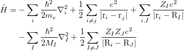$\begin{equation} \begin{split} \hat H = & -\sum _{i}{\frac{\hbar ^2}{2m_ e}}\nabla _ i^2 + \frac{1}{2}\sum _{i\neq {j}}\frac{e^2}{|\text {r}_ i-\text {r}_ j|} + \sum _{i,I}\frac{Z_ Ie^2}{|\text {r}_ i-\text {R}_ I|} \\ & -\sum _{I}{\frac{\hbar ^2}{2M_ I}}\nabla _ I^2 + \frac{1}{2}\sum _{I\neq {J}}\frac{Z_ IZ_ Je^2}{|\text {R}_ i-\text {R}_ J|} \end{split} \end{equation}$

(17)

where electrons are denoted by lower case subscripts and nuclei, with charge $Z_ I$ and mass $M_ I$ , denoted by upper case subscripts. The first term describes the electronic kinetic energy( $\hat T_ e$ ), and the following terms are for electron-electron Coulomb interaction( $\hat V_{int}$ ), electron-nuclear interaction( $\hat V_{ext}$ ), nuclear kinetic energy and nuclear-nuclear Coulomb interaction, seperately. It is assumed the electrons adjust to new atomic positions much faster than the motion of the nuclei (Born-Oppenheimer approximation). Therefore, nuclear kinetic energy can be ignored and nuclear-nuclear Coulomb interaction would be constant. For convenience, Schodinger equation can be rewritten as:

$\begin{equation} (\hat T_ e + \hat V_{int} + \hat V_{ext}) = E\Psi \end{equation}$

(20)

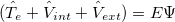
The main problem to solve the equation is that the electronic wavefunction $\Psi$ is a function of 3 $N$ degrees of freedom, which is intractable even for a small nano system. There are many sophisticated methods for solving the many-body Schrodinger equation based on the expansion of the wavefunction in Slater determinants.

$\displaystyle \Psi _0~ ~ ~ =~ ~ ~ \frac{1}{\sqrt {N!}}\left| \begin{array}{cccc} \psi _1(x_1)& \psi _2(x_1)& ...& \psi _ N(x_1)\\ \psi _1(x_2)& \psi _2(x_2)& ...& \psi _ N(x_2)\\ .& .& & .\\ .& .& & .\\ .& .& & .\\ \psi _1(x_ N)& \psi _2(x_ N)& ...& \psi _ N(x_ N)\\ \end{array} \right|$

(21)

where $\psi _ i$ (x) are normalized single-particle wave function for each respective particle. The exchange of any pair of coordinates or any pair of single particle wave functions has the effect of exchanging two rows or columns respectively, which leads to a change of sign of the determinant (anti-symmetry). Thus the ground state wave function $\Psi _0$ is approximated as an anti-symmetrized product of $N$ orthogonal spin orbitals $\psi _ i(x)$ .

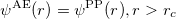
By invoking the variational method, one can derive a set of $N$ -coupled equations for the $N$ spin orbitals. Solution of these equations yields the Hartree-Fock wave function and energy of the system, which are approximations of the exact ones.

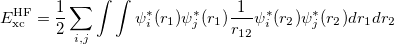
While the simplest one is the Hartree-Fock method, more sophisticated approaches are usually categorized as post-Hartree-Fock methods. However, the problem with these methods is the huge computational effort, which makes it virtually impossible to apply them efficiently to larger, more complex systems.

$\includegraphics[scale=0.8]{chapter2/pdf/HF.png}$

Figure 2.7: Hartree-Fock method illustrated in a simplified flowchart (from Wikipedia).

In computational community, one always refers the electronic structure calculations as ‘ab initio’ or ‘first principles’. In physics, if it starts directly at the level of established laws of physics and does not make assumptions such as empirical model and fitting parameters, it is called first principles, or ab initio, which means ‘from the beginning’ in Latin. The calculation of electronic structure using Schrodinger’s equation within a set of approximations without fitting parameter can be said ’first principles’ or ‘ab initio’ approach. But the term ab initio in quantum chemistry sometimes mainly refers Hartree-Fock and post-Hartree-Fock methods.

Foundation of Density functional theory

Density functional theory (DFT) is so far the most popular method. It is based on two Hohenberg-Kohn theorems ³⁹ as follows:

Theorem I: For any system of interacting particles in an external potential $V_\text {ext}(r)$ , the potential $V_\text {ext}(r)$ is determined uniquely, except for a constant, by the ground state particle density $n_0(r)$ .

Theorem II: A universal functional for the energy $E[n]$ in terms of the density $n(r)$ can be defined, valid for any external potential $V_\text {ext}(r)$ . For any particular potential $V_\text {ext}(r)$ , the exact ground state energy of the system is the global minimum values of this functional, and the density $n(r)$ that minimizes the functional is the exact ground state density $n_0(r)$ .

Therefore, density functional approach can be summarized by the sequence:

$\begin{equation} n(r) ~ \Longrightarrow ~ \Psi (r) ~ \Longrightarrow ~ V(r) \end{equation}$

(22)

Kohn-Sham ansatz

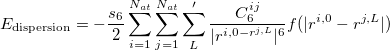
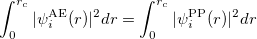
DFT is the most widely used method today for electronic structure calculation because of the approach proposed by Kohn and Sham ⁴⁰: to replace the original many-body problem by an auxiliary independent-particle problem (note that it is still different from Hartree-Fock method). This is an ansatz(a mathematical assumption about the form of an unknown function, which is to facilitate solution of an equation or other problem).

The Kohn-Sham ansatz ⁴⁰ converts the many-body system of the interacting electrons, $\Psi (r_1, r_2, ...)$ , into a set of non-interacting one-body wave functions, $\left\{ \psi _ i(r)\right\}$ and with the same density, $\rho = \sum |\psi _ i(r)|^2$ . The ground state energy of the interacting system $E[\rho ]$ is then the same as the ground state energy of the non-interacting system $E_\textrm {KS}[\rho ]$ , which can be expressed as:

$\begin{equation} \label{eqn:KS} E_\textrm {KS}[\rho ] = E_\textrm {{kinetic}} + \int d^3r[V_\text {ext}(r)\rho (r)] + E_{\textrm{Hartree}}[\rho ] + E_\textrm {xc}[\rho ] \end{equation}$

(23)

The first term is the kinetic energy of the non-interacting electrons and the second term is the potential energy of electrons due to the external field. $E_{\textrm{Hartree}}[\rho ]$ is the direct Coulomb interaction between electrons. The fourth term is the exchange-correlation energy, which is the only unknown term so far. The KS approach involves independent particles but an interacting density. Thus, all the difficult many-body terms are incorporated into the exchange-correlation functional of the density. If the solution of $E_\textrm {xc}[\rho ]$ is available, the KS equation can be solved by self-consistent iteration, which would lead to the exact energy. However, there is no way to obtain the exact form of $E_\textrm {xc}[\rho ]$ . Instead, we have to reasonably approximate it.

$\includegraphics[scale=0.7]{chapter2/pdf/ks.png}$

Figure 2.8: Representation of the self-consistent loop for solution of KS equation (from Quantum Espresso tutorial).

Exchange-correlation energy

The Local Density Approximation (LDA) was firstly proposed by Kohn and Sham, and used in the early works. the exchange-correlation energy density is simply an integral over all space with the $E_\textrm {xc}[\rho ]$ only depending on the local electron density(the same as in a homogeneous electron gas).

$\begin{equation} \label{eqn:lda} E_\textrm {xc}^\textrm {LDA}[\rho ] = \int d^3r \rho (r) E_\textrm {xc}[\rho ] \end{equation}$

(24)

Different interpolation schemes have been proposed for $E_\textrm {xc}[\rho ]$ , like Perdew and Zunger ⁴¹. LDA is the simplest density functional, and was used for a generation in materials science, bus is insufficiently accurate for most chemical purposes. LDA typically overbinds molecules by about 30 kcal/mol, which is an unacceptable error for chemical applications.

DFT has been very popular for calculations in solid-state physics since the 1970s, but only began to be widely accepted by quantum chemists until the 1990s when the exchange-correlation energy approximations were greatly refined. A significant improvement on the performance of DFT was the proposal of Perdew and Wang in 1991 ⁴². They introduced a new functional formula which depends on not only the local density but also on its gradient, better known today as so call Generalized Gradient Approximation (GGA).

$\begin{equation} \label{eqn:gga} E_\textrm {xc}^\textrm {GGA}[\rho ] = \int d^3r \rho (r) E_\textrm {xc}[\rho , \nabla \rho , ] \end{equation}$

(25)

GGA improves the shortcomings of LDA’s poor description of strong inhomogeneous system. Many different reformulations and extensions of GGA have been proposed and tested over the years. Traditionally, physicists favor a non-empirical approach, deriving approximations from quantum mechanics and avoiding fitting to specific finite systems. One of the physics type of GGA functionals is the Perdew-Burke-Ernzerhof (PBE) ⁴³, which is widely used in material sciences (and also in this thesis!). On the other hand, chemists typically use a few or several dozen parameters to improve the accuracy on a limited class of molecules, like LYP ⁴⁴ and its revised version BLYP functional ⁴⁵, which has smaller errors for main-group organic molecule energetics than PBE, but does badly for the correlation energy of metals.

Currently, the key development in DFT is to obtain more accurate $E_\textrm {xc}[\rho ]$ functionals. Towards this target, the progresses are very diverse and rapid. Here I just list a few directions according to my research interest. I strongly recommend the excellent review by Burke ⁴⁶ for details.

Semi-local functionals. Universal GGAs such PBE work for a wide range of systems, but they are still limited in accuracy. One approach is to devise GGAs that are specialized for certain classes of compounds. PBEsol ⁴⁷ GGA is an example: it recovers the original gradient expansion for exchange, and its correlation piece is adjusted to reproduce jullium surface energies accurately. Due to its diminished gradient dependence, PBEsol is biased towards solids and yields better lattice constants and other equilibrium properties of densely packed solids than PBE. However, it is generally less accurate for molecular bond energies.

Hybrid functionals. One significant failure of DFT is the systematic underestimation of the fundamental gaps of semiconductor and insulators. In the early 1990s, hybrids were introduced by Becke ⁴⁸, replacing a fraction of GGA exchange with HF exchange,

$\begin{equation} \label{eq:hf} E_\textrm {xc}^\textrm {HF} = \frac{1}{2}\sum _{i,j}\int \int \psi _ i^*(r_1) \psi _ j^*(r_1) \frac{1}{r_{12}} \psi _ i^*(r_2) \psi _ j^*(r_2) dr_1dr_2 \end{equation}$

(26)

A practical way is to use a hybrid, but the exchange term as orbital dependent, via generalized KS theory. Thus the hybrid version of PBE and BLYP were proposed as PBE0 ⁴⁹, HSE ⁵⁰ and B3LYP ⁴⁸.

B3LYP is currently the most popular form used by chemists. The formulation is based on Becke 88 exchange functional and LYP correlation functional (Becke, three-parameter, Lee-Yang-Parr):

$\begin{equation} \label{eq:b3lyp} E_\textrm {xc}^\textrm {B3LYP} = E_\textrm {xc}^\textrm {LDA} + a_0(E_ x^\textrm {HF} - E_ x^\textrm {LDA}) + a_ x(E_ x^\textrm {B88} - E_ x^\textrm {LDA}) + a_ c(E_ c^\textrm {LYP} - E_ c^\textrm {VWN}) \end{equation}$

(27)

where $a_0$ =0.20, $a_ x$ =0.72, $a_ c$ =0.81. $E_ x^\text {B88}$ and $E_ c^\text {LYP}$ are from Becke 88 and LYP functional, $E_ c^\text {VWN}$ is from the VWN-LDA functional for correlation.

If PBE mixes 0.25 HF exchange, it would lead to PBE0 functional,

$\begin{equation} \label{eqn:pbe0} E_\textrm {xc}^\textrm {PBE0} = 0.25~ E_\text {x}^\text {HF} + 0.75~ E_\text {x}^\text {PBE} + E_\text {c}^\text {PBE} \end{equation}$

(28)

HSE uses an error function screened Columb potential to calculate the exchange portion of the energy in order to improve the computational efficiency, especially for metallic systems.

$\begin{equation} \label{eqn:hse} E_\textrm {xc}^\textrm {HSE} = 0.25~ E_\text {x}^\text {SR}(\mu ) + 0.75~ E_\text {x}^\text {PBE,SR}(\mu ) + E_\text {x}^\text {PBE,LR}(\mu )+E_\text {c}^\text {PBE} \end{equation}$

(29)

The separation of the electron-electron interaction into a short- and long-ranged part, labeled SR and LR respectively, is realized only in the exchange interactions.

Dispersion effects. DFT is notoriously known to poorly describe long-range dispersion effects. Due to their dependence on the local density, the semi-local functionals cannot account for XC effects due to the presence of electrons in remote parts of a molecule. There are many attempts to correct this by adding a vdW attraction between the nuclei to the nuclear potential energy ( $E_\text {dispersion}$ )

$\begin{equation} \label{eqn:hse} E_\text {DFT-D} = E_\text {KS} + E_\text {dispersion} \end{equation}$

(30)

and $E_\text {dispersion}$ can be derived from a empirical force field. For instance, in the DFT-D2 methond of Grimme ⁵¹, it is described via a simple pair-wise force field,

$\begin{equation} E_\text {dispersion} = -\frac{s_6}{2} \sum _{i=1}^{N_{at}} \sum _{j=1}^{N_{at}} \sum _ L^{\prime } \frac{C_6^{ij}}{|r^{i,0 - r^{j,L}}|^6} f(|r^{i,0} - r^{j,L}|) \end{equation}$

(31)

where the summations are over all atoms $N_{at}$ and all translations of the unit cell $L = (l_1, l_2, l_3)$ , the prime indicates that $i\neq j$ for $L\neq 0$ , $s_6$ is a global scaling factor, $C_6^{ij}$ denotes the dispersion coefficient for the atom pair $ij$ , $r^{i,L}$ is a position vector of atom $i$ after performing $L$ translations. The term $f(r^{ij})$ is a damping function,

$\begin{equation} f(r^{ij}) = -\frac{1}{1+e^{-d(r^{ij}/R_0^{ij}-1)}} \end{equation}$

(32)

where $R_0$ denotes the vdW radii. Dispersion coefficient and vdW radii are two parameters well defined for each element from the empirical force field. The Combination rules for dispersion coefficient $C_6^{ij}$ and vdW radii $R_0^{ij}$ are

$\begin{equation} C_6^{ij}=\sqrt {C_6^ i C_6^ j} \end{equation}$

(33)

$\begin{equation} R_0^{ij}=\sqrt {R_0^ i + R_0^ j} \end{equation}$

(34)

DFT with dispersion functional usually gives accurate results for a restricted class of compounds. But the accuracy strongly depends on the quality of the force fields, thus it can not be transferable. A fully non-local non-empirical dispersion correction to GGAs was proposed as so called vdW-DF functional ⁵². However, its original formulation requires large computational cost. It was recently improved by using the algorithm of Roman-Perez and Soler which transforms the double real space integral to reciprocal space and therefore could largely reduce the computational effort ^{53; 54}.

Orbital-dependent functionals. Another major problem of standard LDAs and GGAs is that they could not describe the system when the electrons tend to be localized and strongly interacting, such as transition metal oxides and rare earth elements and compounds. LDA+U ⁵⁵ is a very popular method to remedy this issue. LDA+U stands for methods that involve LDA- or GGA-type calculations coupled with an additional orbital-dependent interaction. The additional interactions is usually considered only for high localized atomic-like orbitals on the same site, as the ‘U’ interactions in Hubbard models ⁵⁵.

$\begin{equation} E^ U = \frac{1}{2} U \sum _{i \neq j} n_ in_ j \end{equation}$

(35)

There the functional can be rewritten as:

$\begin{equation} E^\text {LDA+U} = E^\text {LDA} + E^ U + E^\text {dc} \end{equation}$

(36)

The $E^\text {dc}$ is called the double counting term, to remove the energy contribution of these orbitals which is twice introduced by the Hubbard term. $E^\text {dc}$ can be approximated as mean-field value of the Hubbard term. The final term of $E^\text {LDA+U}$ is:

$\begin{equation} E^\text {LDA+U} = E^\text {LDA} + \frac{1}{2} U \sum _{i \neq j} n_ in_ j - UN(N-1)/2 \end{equation}$

(37)

where $N=\sum _ i n_ i$ . The effect of U term is to shift the localized orbitals relative to the other orbitals, to correct errors in the usual LDA or GGA calculations. However, I would like to mention that even if LDA or GGA functional describe poorly the electronic properties of the localized orbitals, the energetics and structural properties are adequately reproduced. The U parameter is often taken from constrained density functional calculations so that the theories do not contain adjustable parameters.

Basis set

To practically solve the KS equation without any information from the experiments, one should start with a set of functions to create the wavefuction, which is called basis set. Here I introduce two types of basis sets, plane wave and atomic orbital.

Plane waves. Plane wave basis set is the most natural solution for periodic crystals where they provide intuitive understanding and simple algorithms for practical calculations. Its main disadvantage is that a huge number of plane waves might be required to describe the dramatic change of the wavefunction (for instance, the wavefunction from the deep core electrons to valence electrons). There are several ways to overcome this problem - the LAPW method, Projector Augmented Wave method, pseudopotential method.

Plane wave is perfect fit for periodic boundary conditions. Molecules and surfaces can be treated in an apporximate model by inseting vacuum layers. However, a very large number of plane waves will be spent. Therefore, a more economical way is to consider another type of basis set based on localized orbitals.

Linear combination of atomic orbitals(LCAO). LCAO defines atom-centered orbitals as a product of the angular(Y $_{lm}$ ) and radia ( $\chi (r)$ ) parts:

$\begin{equation} \psi _ i(r)=Y_{lm}\chi (|r|) \end{equation}$

(38)

where the radial part is a linear combination of Slater-type functions or Gaussian-type functions. Slater oribtals are more accurate but requires much more computational cost. Gaussian functions are usually preferred.

Pseudopotentials

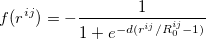
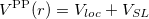
A very important idea for efficient implementation of DFT is the pseudopotential. In practice, electrons are usually separated into core and valence electrons. The core electrons are usually chemically inert, and do not contribute to bonding. There is no need to treat them explicitly. Therefore, pseudopotential can be constructed to frozen the core electrons while only consider the chemically active valence electrons. A good pseudopotential should satisfy the following rules:

1) The pseudo wave functions should be identical to the all-electron wave functions outside the cut-off radius( $r_ c$ ), as shown in Fig. 2.9.

$\begin{equation} \psi ^\text {AE}(r)=\psi ^\text {PP}(r), r>r_ c \end{equation}$

(39)

2) The eigenvalues should be conserved.

$\begin{equation} \varepsilon _ i^\text {AE}(r)=\varepsilon _ i^\text {PP} \end{equation}$

(40)

3) The total charge of each pseudo wave function should equal the charge of the all-electron wave function.

$\begin{equation} \int _0^{r_ c}|\psi _ i^\text {AE}(r)|^2dr = \int _0^{r_ c}|\psi _ i^\text {PP}(r)|^2dr \end{equation}$

(41)

4) The scattering properties of the pseudopotential should be conserved.

According norm-conserving condition. The pseudopotential $V_ i(r)$ can be split into a local part, long-ranged and behaving like $-Z_ ve^2/r$ for $r\rightarrow \infty$ , and a short-ranged semilocal term:

$\begin{equation} \label{eq:pp} V^\text {PP}(r) = V_{loc} + V_{SL} \end{equation}$

(42)

where $V_{loc}(r)$ is a radial function, and the semi-local part is the deviation from the all-electron potential inside the core region,

The pseudopotential reproduces the true potential outside the core region, but is much smoother inside the core. The oscillations of the electron wave function inside the core region are eliminated by the pseudopotential. This is a great advantage for numerical calculations. A further approximation, the ultrasoft pseudo-potential ⁵⁶, uses more than one projector for each momentum, and further smooths the electron wave function.

$\includegraphics[scale=0.5]{chapter2/pdf/pp.png}$

Figure 2.9: Comparison of a wave function in the Coulomb potential of the nucleus (blue) to the one in the pseudopotential (from wikipedia).

The projector augmented wave (PAW) method ⁵⁷ is a general approach to solution of the electronic structure. The PAW approach introduces projectors and auxiliary localized functions, like ultrasoft type method. However, it also keeps the full all-electron wavefunction in a form similar to the general OPW expression.

Brillouin zone sampling

A 3D periodic crystal should contain an infinite number of electrons. Yet, it is possible to consider only one unit cell by introducing the reciprocal lattice according to Bloch theorem:

$\begin{equation} \label{eq:bloch} \psi _{i\text {k}}(r) = e^{i\text {k}r}\cdot w_\text {k}(r) = e^{i\text {k}r} \sum _\text {K}C_\text {k+K}\cdot e^{i\text {k}r} \end{equation}$

(43)

Bloch theorem states that the eigenstates of a periodic Hamiltonian can be written as a product of a periodic function with a plane wave of momentum k restricted to be in the first Brillouin Zone (BZ). Therefore the KS equation must be solved for each point of the fist BZ.

For many properties such as the total energies, it is essential to integrate over k throughout the BZ. An intrinsic property of a crystal expressed ’per unit cell’ is an average over k divided by the number of values $N_ k$ . For a function $f_ i(\bf k)$ , where $i$ denotes the discrete band index, the average value is:

$\begin{equation} f_ i = \frac{1}{N_ k}\sum _ kf_ i(k) \rightarrow \frac{\Omega _\text {cell}}{(2\pi )^ d}\int _\text {BZ}dkf_ i(k) \end{equation}$

(44)

where $(2\pi )^ d/\Omega _\text {cell}$ is the volume of a primitive cell of the BZ.

In numerical calculation, we cannot go thorough all the BZ. In practice, we can only sample a finite set of k-points. Generally, metals need many more k-points than for insulators and semiconductors to obtain the converged energy. Currently, the most popular meshing strategy is proposed by Monkhorst and Pack ⁵⁸. They defined a uniform set of special k-points as:

$\begin{equation} \label{eq:mp} \text {\bf k} = \bf u_ p{b_1} + u_ rb_2 + u_ sb_3 \end{equation}$

(45)

where $\bf b_1, b_2, b_3$ are the reciprocal lattice vectors, and $u_ p, u_ r, u_ s$ are numbers from the sequence:

$\begin{equation} \label{eq:mp2} {\bf u_ r} = (r2-q-1)/2q~ ~ ~ ~ ~ ~ (r=1,2,3,...q) \end{equation}$

(46)

The total number of k-points is $q^3$ , but the number of the irreducible k-points can be decreased a lot by symmetry.