Crystal Structure Prediction and its Application in Earth and Materials Sciences: Semi-empirical potentials

2.2 Semi-empirical potentials

One can also calculate the electronic wavefunction for fixed atomic positions, and then use different approximations to parametrize analytic functional forms from quantum-mechanical arguments. The implementaion of semi–empirical potentials can be in many forms, depending on the nature of the system. Here we just take the Embedded Atom Model (EAM) ³⁸ as an illustration. EAM treats the bonding in metallic systems based on the concept of local electron density, which allows consideration of the strength of individual bonds on the local environment for simulation of surfaces and defects.

The potential energy of an atom $i$ is given by

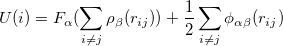$\begin{equation} \label{eam} U(i) = F_{\alpha }(\sum _{i{\neq }j} \rho _{\beta }(r_{ij})) + \frac{1}{2} \sum _{i{\neq }j} \phi _{\alpha \beta } (r_{ij}) \end{equation}$

(15)

where $r_{ij}$ is the distance between atoms i and j, $\phi _{\alpha \beta }$ is a pair-wise potential function, $\rho _{\beta }$ is the contribution to the electron density from atom $j$ of type $\beta$ at the location of atom $i$ , and $F$ is an embedding function that sums over the energy associated with placing an atom in the electron environment $\rho$ . $F$ could have many forms. Some authors derive functions and parameters from first principles calculations, while others guess the functions and fit parameters to experimental data. Generally these functions are provided in a tabularized format, interpolated by cubic splines ³⁸.