- Required Reading: Lab 12. It is hard to understand software/equipment without first seeing and playing with it, but insofar as possible you should be ready to use the Clea Stellar Spectra software and spectrometers including the Project Star Spectrometer.
- Read the Startup Presentation.
- Read the Post Mortem. Better before than after actually.
- Read a sufficient amount of the articles linked to the following terms etc. so that you can define and/or understand the terms etc. at the level of our class: absorption line spectrum, atomic spectral lines, Clea Stellar Spectra software, color index (AKA color), diffraction, diffraction grating, diffraction grating formula, electromagnetic spectrum, emission line spectrum, Fraunhofer lines, gas-discharge lamp, sodium-vapor lamp, Grotrian diagram, Hertzsprung-Russell diagram, hydrogen Balmer lines, incandescent light bulb, Kirchhoff's 3 laws of spectroscopy, light, luminosity, main sequence, Moore & Merrill Grotrian diagrams, Na D lines, OBAFGKM stellar classification, photopic vision, photosphere, objective-prism spectroscopy, prism, Project Star Spectrometer, Schmidt camera (AKA Schmidt telescope), scotopic vision, spectral lines, spectral types, spectrometer (AKA spectroscope), spectroscopy, stellar classification, visible light, white light, Wien's law, WINSCO spectrometer.

Caption: A schematic Hertzsprung-Russell (HR) diagram with color index (AKA color) B-V along the lower horizontal axis, spectral type along the upper horizontal axis, and absolute magnitude in V along the vertical axis.
Absolute magnitude in V is a proxy for luminosity (total power integrated over all wavelength).
The bands on the diagram of the luminosity classes are:
-
0 := hypergiants See Wikipedia: List of most massive stars,
where the current record massive star
is about 300 M_Suns.
Ia := supergiants
Ib := bright giants
III := giants
IV := subgiants
V := main-sequence stars which are also called dwarf stars, but that now seems a disfavored term.
VI := subdwarf stars
VII := white dwarfs
Credit/Permission: © User:Rursus, 2007 / Creative Commons CC BY-SA 3.0.
Image linked to Wikipedia.
Supplementary Lab Preparation: The items are often alternatives to the required preparation.
- Bennett, p. 149--157, 163--171 on light and p. 518--538 on stars.
- IAL 6: Electromagnetic Radiation, IAL 7: Spectra, and IAL 20: Star Basics II.
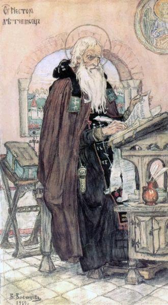
Caption: St. Nestor the Chronicler (c. 1056--c. 1114), St. Vladimir's Cathedral, Kiev, Ukraine.
At his studies.
Credit/Permission: Viktor Vasnetsov (1848--1926), 1919 (uploaded to Wikipedia by User:Butko, 2006) / Public domain.
Image linked to Wikipedia.
The quiz might be omitted if it's not feasible or convenient. The students may or may not be informed ahead of time of quiz omission depending on the circumstances.
The quizzes in total are 40 % of the course grade. However, only the top five quiz marks are counted.
In preparing for a quiz, go over the Required Lab Preparation.
The Supplementary Lab Preparation (see above) could help, but is only suggested if you feel you need more than the required Required Lab Preparation.
There is no end to the studying you can do, but it is only a short quiz.
One to two hours prep should suffice.
There will be 10 or so questions and the time will be 10 or so minutes.
The questions will range from quite easy to challenging.
-
Some of the questions will be thinking questions. You will have to reason your way
to the answers.
The solutions might be posted at Stellar Spectra: Quiz Solutions. after the quiz is given. Whether they are or not depends on the circumstances of each individual semester.
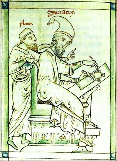
Caption: Plato (428/427--348/347 BCE) and Socrates (circa 469--399 BCE) in a Medieval image.
Here the disciple seems to be instructing the master/mentor using the Socratic method.
The basic pose is much like in intro labs.
Credit/Permission: Medieval artist, Middle Ages (probably 1000--1400) (uploaded to Wikipedia by User:Tomisti, 2007) / Public domain.
Image linked to Wikipedia.
- Read a sufficient amount of the articles linked to the following terms etc. so that you can define and/or understand the terms etc. at the level of our class: absorption line spectrum, atomic spectral lines, Clea Stellar Spectra software, color index (AKA color), diffraction, diffraction grating, diffraction grating formula, electromagnetic spectrum, emission line spectrum, Fraunhofer lines, gas-discharge lamp, sodium-vapor lamp, Grotrian diagram, Hertzsprung-Russell diagram, hydrogen Balmer lines, incandescent light bulb, Kirchhoff's 3 laws of spectroscopy, light, luminosity, main sequence, Moore & Merrill Grotrian diagrams, Na D lines, OBAFGKM stellar classification, photopic vision, photosphere, objective-prism spectroscopy, prism, Project Star Spectrometer, Schmidt camera (AKA Schmidt telescope), scotopic vision, spectral lines, spectral types, spectrometer (AKA spectroscope), spectroscopy, stellar classification, visible light, white light, Wien's law, WINSCO spectrometer.


- Check as needed:
- Prof. Smith's instructor notes
- This is an inside lab, and so no need to check the
weather at
NWS
7-day forecast, Las Vegas, NV and/or by personal visual inspection at/during the lab period.
- You will need to set out the
spectrometers
(both the
Project Star Spectrometer
and the
WINSCO spectrometer),
gas-discharge lamp
for sodium (Na)),
and
incandescent light bulb lamp.
- Make sure the Fraunhofer spectrum
chart is displayed on the wall
(see also Wikipedia: Fraunhofer spectrum)
and Clea Stellar Spectra software
is on the computers
(but it really ought to be).
- Hand back old reports and quizzes.
- Start at 7:30 pm sharp.
- Give tonight's agenda: quiz, post mortem on the last lab,
Startup Presentation, lab. Be brief.
- Then give the quiz. It will be 10 minutes or so.
Late arrivals have to write the quiz at the tables in the hall.
- Give the Post Mortem of the last lab. Be brief.
- Then tell them to form new groups,
report to a computer,
launch Firefox,
click down the chain
Jeffery astlab on bookmarks,
Lab Schedule,
tonight's lab,
and srcoll down past the foxes.

Caption: "Red foxes (Vulpes vulpes) at the British Wildlife Centre, Horne, Surrey, England." (Slightly edited.)
Credit/Permission: © Keven Law, 2008 / Creative Commons CC BY-SA 2.0.
Image linked to Wikipedia.
- Objectives: The objectives are to learn how
emission line spectra,
absorption line spectra,
and
continuous spectra
are formed, and to learn some basics of analyzing
stellar spectra.
- Spectral Lines:
- The electrons
in atoms
and
molecules
are in discrete (i.e., quantized) internal energy states which are called
energy levels.
Each atom, molecule, and ion (a non-neutral atom or molecule) has its own unique set of energy levels.
The energy levels are illustrated in Grotrian diagrams.
Examples of Grotrian diagrams are found at Jeffery: Grotrian diagrams
The H I (i.e., neutral hydrogen atom) Grotrian diagram is displayed below.
The hydrogen atom is the simplest of all atoms, and so its Grotrian diagram is the simplest of all Grotrian diagrams.
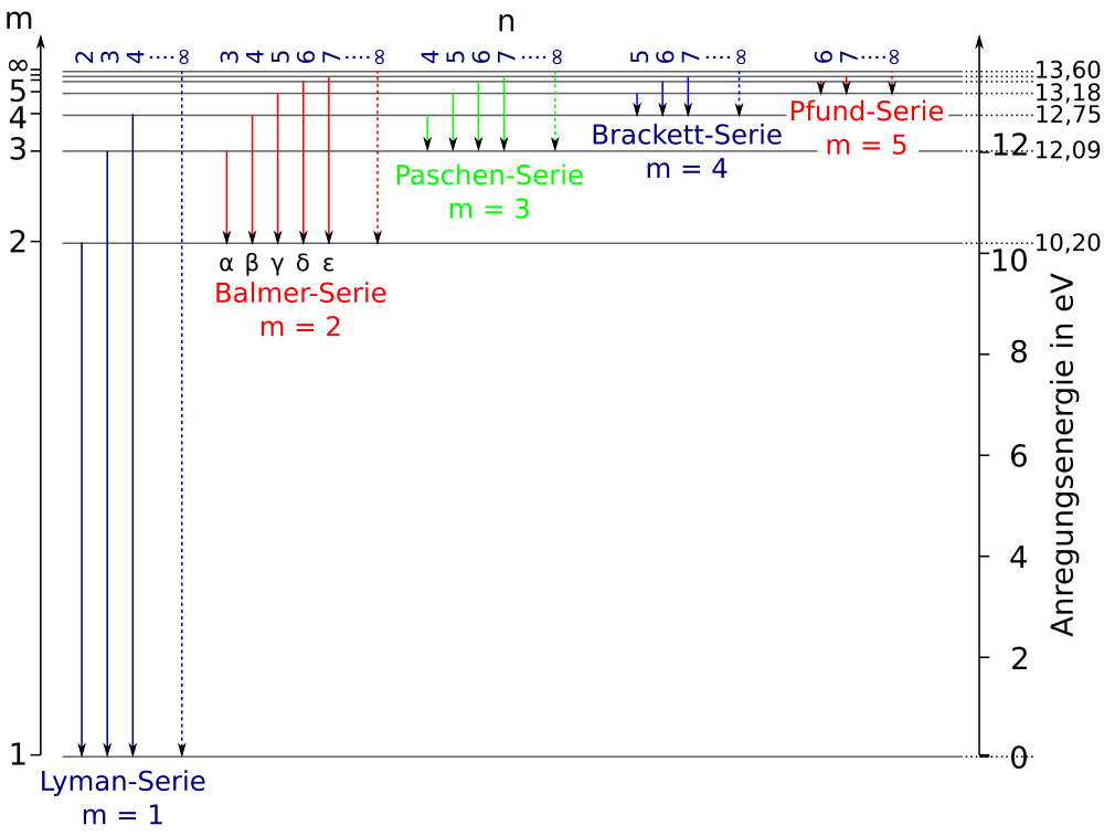
Caption: H I Grotrian diagram.
Below, we consider the energy levels and then the atomic line transitions for the hydrogen atom.
For energy levels, we use ideal hydrogen atom values. For atomic line transitions, we use values tabulated by the National Institute of Science & Technnology (NIST) (formerly the National Bureau of Standards (NBS)) (Wiese et al. 1966, p. 2; Wiese et al. 1966, p. 2, online).
The formula for energies of the energy levels of the ideal hydrogen atom (i.e., the hydrogen atom calculated without any perturbation corrections included, but using the correct reduced mass) is
E_n = -E_ryd*(μ/m_e)/n**2

    = -(13.5982 ... eV)/n**2  ,


  where
  the Rydberg energy = 13.60569253(30) eV,
  the reduced Rydberg energy = 13.5982 ... eV,
  the electron reduced mass μ=m_e/(1+m_e/m_p)=(0.9994 ...)*m_e,
  the electron rest-mass energy m_e=0.510998910(13) MeV,
  the proton rest-mass energy m_p=938.272046(21) MeV,
  energy is in electron-volts (eV) (1 MeV=10**6 eV),
  and
  n is the principal quantum number
    which runs 1, 2, 3, ... in order of increasing energy level energy for the hydrogen atom.
The zero point for the energies is zero energy of the continuum of energy states available to free (i.e., unbound) electrons.
To get the energy measured from the ground state of the hydrogen atom, one uses formula E_grd_n = E_n - E_1.
To get the energy of a particular transition, one uses the formula E = E_n_upper - E_n_lower.
In the table below, we show the hydrogen atom energy levels.
 ----------------------------------------------------
 Table:  Energy Levels of the Ideal Hydrogen Atom
 ----------------------------------------------------
   n      E_n           E_grd_n
          (eV)            (eV)
 ----------------------------------------------------

   1    -13.598 ...     0.0000 ...
   2    -3.3995 ...    10.1987 ...
   3    -1.5109 ...    12.0873 ...
   4    -0.8498 ...    12.7483 ...
   5    -0.5439 ...    13.0543 ...
   6    -0.3777 ...    13.2205 ...
   7    -0.2775 ...    13.3207 ...
   ∞     0             13.5982 ...
 ----------------------------------------------------
The atomic line transitions for the hydrogen atom are tabulated below.
-
Table: Atomic Hydrogen Spectral Series
- Lyman series n ≥ 2 → 1 transitions
- Balmer series n ≥ 3 → n=2 transitions
- Paschen series n ≥ 4 → 3 transitions
- Brackett series n ≥ 5 → 4 transitions
- Pfund series n ≥ 6 → 5 transitions
- Humphreys series n ≥ 7 → 6 transitions
- No name series n ≥ 8 → n ≥ 7 transitions
Credit/Permission: © User:Kiko2000, User:Cepheiden, 2000 / Creative Commons CC BY-SA 3.0.
Image linked to Wikipedia.
- Transitions
between the energy levels
can absorb or emit
light
(AKA electromagnetic radiation)
in the form of photons.
The wavelength of photons from a single transitions is very narrow: e.g., much, much smaller than the wavelength band of visible light.
The most prominent of transitions are often illustrated on Grotrian diagrams
The H I Grotrian diagram shown above illustrates the hydrogen spectral series.
The atomic hydrogen spectral series are directly observed when electromagnetic radiation (EMR) from a dilute neutral atomic hydrogen gas is dispersed into what is called a line spectrum.
The atomic hydrogen spectral series image line spectrum (as opposed to an intensity line spectrum) is illustrated in the cartoon below.
- Lyman series (Ly) n ≥ 2 → 1 transitions
- Balmer series (Ba) n ≥ 3 → n=2 transitions
- Paschen series (Pa) n ≥ 4 → 3 transitions
- Brackett series (Br) n ≥ 5 → 4 transitions
- Pfund series (Pf) n ≥ 6 → 5 transitions
- Humphreys series (Hu) n ≥ 7 → 6 transitions
- No name series n ≥ 8 → n ≥ 7 transitions
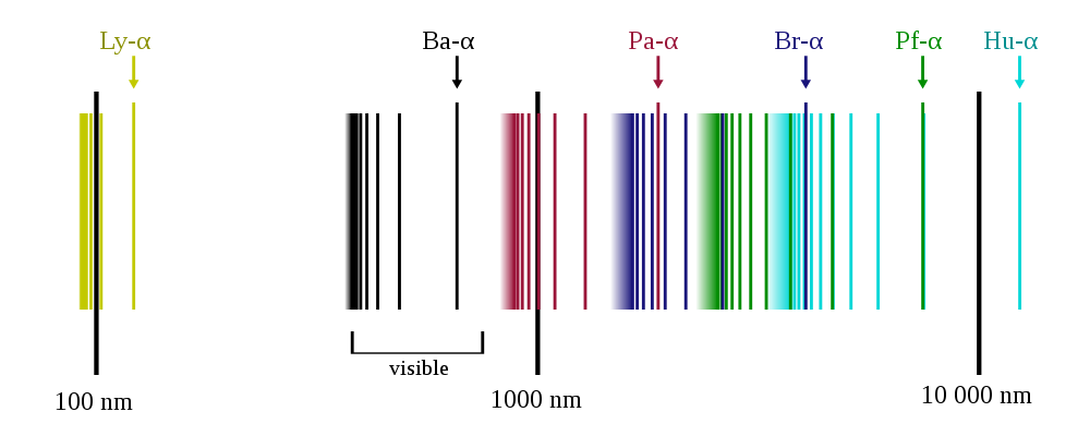
Caption: A cartoon of the image line spectrum of hydrogen (i.e., atomic hydrogen spectral series) shown on a logarithmic scale.
This line spectrum is observed when electromagnetic radiation (EMR) from a dilute neutral atomic hydrogen gas is dispersed into what is called a line spectrum.
The atomic hydrogen spectral series are detailed in the table below.
Table: Atomic Hydrogen Spectral Series
Credit/Permission: © User:OrangeDog, 2009 / Creative Commons CC BY-SA 3.0.
Image linked to Wikipedia.
- Since the energy levels
are uniquely quantized for each
atom,
molecule,
and ion, the
transitions
are uniquely quantized.
The line spectrum from the transitions is a unique identifier of the atom, molecule, or ion.
- The spectrum of a
atom,
molecule,
or ion.
is called a
line spectrum since
when light consisting only of light from
transitions is
dispersed
by prism
or diffraction grating,
you get a spectrum of lines rather than
continuous spectrum
(AKA continuum) as
with, e.g., white light.
The lines are called spectral lines.
- Below is the visible light
spectrum of a dilute neutral atomic hydrogen gas.
The spectral lines are called the Balmer lines.
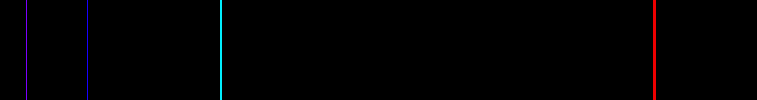
Caption: The first four hydrogen Balmer lines (which are the main visible of atomic spectral lines of atomic hydrogen gas). The Balmer lines are part of the overall hydrogen spectral series.
Going blueward, the lines are Halpha, Hbeta, Hgamma, and Hdelta. The Halpha line is ubiquitous in astrophysical images: it gives that nebulous pink color in true color images of gaseous nebulae.
Note the Balmer lines are for an atomic hydrogen gas (i.e., a gas of hydrogen atoms) and not a molecular hydrogen gas (i.e., a gas of hydrogen molecules H_2).
If you have any relatively low-density hot gas, then it will emit a emission line spectrum, not a continuous spectrum like that of white light. The lines of an emission line spectrum are all you get when the light from the gas is dispersed through a prism.
Such emission line spectra are used to identify atoms and molecules in the technique known as spectroscopy.
Credit/Permission: Merikanto, circa or before 2006 / Public domain.
Image linked to Wikipedia.
- Atomic hydrogen has a rather
simple line spectrum.
Neutral Iron (Fe) has a much more complex one as the figure below illustrates.

Caption: Visible light emission line spectrum of neutral iron.
Credit/Permission: User:Teravolt, 2010 / Public domain.
Image linked to Wikipedia.
- The electrons
in atoms
and
molecules
are in discrete (i.e., quantized) internal energy states which are called
energy levels.
- Continuous Spectra
and Line Spectra:
The atomic line spectra just shown are emission line spectra.
They arise from low-density gases, where there are NOT sufficient processes to produce a continuous spectrum where there is electromagnetic radiation (EMR) at every wavelength over a wide wavelength band.
You can have emission line spectra superimposed on a continuous spectrum.
A pure continuous spectrum is produced by a dense radiator.
If the radiator is all at one temperature, you get a blackbody spectrum which has very simple functional form which is only a function of temperature and wavelength.
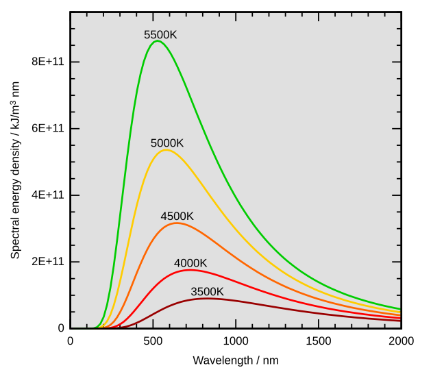
Caption: Blackbody spectra for a range of Kelvin temperatures
T=5500 K is not far from the Sun's effective temperature 5778 K.
The effective temperature of a body is the surface temperature it would have if it radiated exactly like a blackbody radiator and had exactly the same luminosity as it actually has.
The effective temperature of the Sun is the same to within significant figures as the temperature 5800 K of a blackbody spectrum fitted to the actual solar spectrum.
Credit/Permission: © 4C / Creative Commons CC BY-SA 3.0.
Image linked to Wikipedia.
The wavelength at which the Blackbody spectrum reaches its maximum is given by The wavelength peak of a blackbody spectrum intensity (energy/(area*steradian*time*wavelength)) is determined by Wien's law (AKA Wien's displacement law).

Caption: Wien's law illustrated.
Wien's law and its inverse are
         2897.7685(51) μm*K   2.8977685(51)*10**6 nm*K
 λ_max = ------------------ = ------------------------
                 T                       T

 and

     2897.7685(51) μm*K   2.8977685(51)*10**6 nm*K
 T = ------------------ = ------------------------  ,
           λ_max                  λ_max
where temperature is in kelvins.
If one can find the λ_max for a star, then the inverse Wien's law can be used to determine its approximate photosphere temperature.
For example, a very hot star has λ_max = 0.075 μm, and so has T_photosphere ≅ 40,000 K.
For the lab question using Wien's law it is convenient to have the luminosity function for the human eye: see just below.
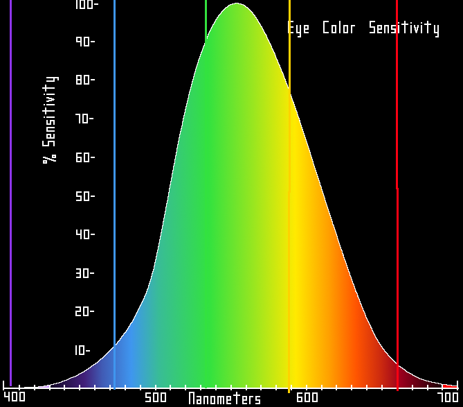
Caption: The psychophysical sensitivity of the average human eye (i.e., luminosity function).
The vertical scale is just relative to maximum sensitivity set to 100 %.
The colored vertical lines are at the wavelengths of some common laser colors. The yellow line is the 589,590 nm sodium D lines.
This diagram is for photopic vision (i.e., human eye vision under well lit condtions).
There is another sensitivity curve for scotopic vision (i.e., human eye vision under poorly lit condtions).
Credit: User:Skatebiker, 2010 / Public domain.
Image linked to Wikipedia.
- Stellar Spectra:
- Formation of Absorption Line Spectra:
Stellar spectra approximate blackbody spectra.
The blackbody-like spectra are generated at the stellar photosphere which is often referred to as the stellar surface.
But above the photosphere, there is a low-density stellar atmosphere that is usually at a lower temperature than the photosphere.
This low-density stellar atmosphere absorbs in the atomic spectral lines molecular spectral lines causing dark absorption lines in the stellar spectra just where bright lines appear in an emission spectrum.
The absorption line spectrum of atom, molecule, or ion is a unique identifier of that species.
The formation of an absorption line spectrum is illustrated in the figure below.

Caption: The formation of an absorption line spectrum.
The atoms, molecules, and/or ions in the low-density stellar atmosphere above the photosphere are colder (i.e., less excited) than the photosphere. They will absorb the photospheric emission in their lines.
Thus, they create dark lines that form an absorption line spectrum.
Credit/Permission: NASA, NASA: Imagine the Universe, before or circa 2009 / Public domain.
Of course, Stellar spectra can be immensely complex because many kinds of atoms, molecules, or ions occur in stellar atmospheres.
- Hydrogen Line Spectrum:
Atomic hydrogen lines are nearly ubiquitous in universe because hydrogen dominant element in nearly all stars.
So it is understandable that atomic hydrogen lines are common in stars and are usually their most recognizable atomic lines.
The figure below show the primordial nebula solar composition which is approximately the universal composition of the cosmic time.

Caption: A plot of the primordial nebula solar composition or, for short, the solar composition.
It's not exactly the composition of the Sun or any particular Solar System astro-body, but rather the best-calculated composition for the primordial nebula out of which the Solar System formed.
It is obtained from observations of the solar photosphere and from primitive meteorites: i.e., meteorites that seem to have undergone little chemical processing since the solar system formation.
The plot is a semi-log graph with the vertical axis being logarithmic and the horizontal axis being atomic number.
The plot is by mass fraction.
Many solar composition plots are by number fraction.
As one can see, hydrogen and helium are the dominant species.
Once you get to atomic numbers greater than copper, the abundances become small.
The data are from Asplund et al. (2005).
The cosmic composition of present cosmic time is believed to be similar throughout the local universe. Approximately by mass fraction: Approximately by mass fraction:
         H (hydrogen)  74 + (Z-2) %

         He (helium)   24 + (Z-2) %

         metallicity    Z %

    (see Wikipedia:  Abundance of chemical elements:  Abundance of elements in the universe).
In astro-jargon, metallicity is the metals collectively. The metals are everything that is NOT H and He.
In the solar composition and in the local universe, Z is about 2 %, but Z varies wildly between stars even in one galaxy from low of less than about 10**(-6) to about 4 %???.
In non-stellar astro-bodies like rocky planets, Z can go to nearly 100 %, of course.
The record low-metallicity in stars as of 2013 is/was Caffau's star which is located in the Galactic halo---the capital G means this is the Galactic halo of the Milky Way (AKA the Galaxy with a capital G).
The relative abundances among the metals vary much less strongly than the the overall metallicity since the metals are produced by the same processes in, mainly, stars and supernovae. It is amount of such production that determines the overall metallicity.
Credit/Permission: David Jeffery, circa 2010 / Own work.
- The Solar Spectrum:
The solar spectrum is the prototype stellar spectrum, of course.
An image (or color) solar spectrum is illustrated in the figure below.
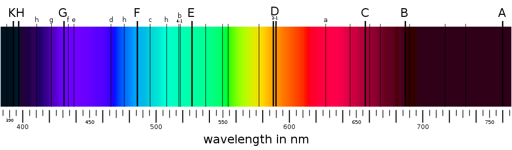
Caption: Solar spectrum with the Fraunhofer lines from range 380--710 nm (i.e., approximately the visible band.
I think the spectrum may be just a simulated spectrum.
The Solar spectrum is the most famous absorption line spectrum. The absorption lines are tabulated at Wikipedia: Fraunhofer lines: Naming.
I think the spectrum may be just a simulated spectrum.
Some of the absorption lines in the solar spectrum are telluric lines---they are caused by absorption in the Earth's atmosphere.
Telluric lines are tradtionally regarded as part of the Fraunhofer lines because Joseph von Fraunhofer (1787--1826) discovered them---but William Hyde Wollaston (1766--1828) discovered them first in 1802.
Telluric lines are usually removed in modern stellar spectroscopy because they are NOT intrinsic to the nature of stars, and so tell nothing about stars.
Credit/Permission: User:MaureenV, circa or before 2009 (uploaded to Wikipedia by User:Cepheiden, 2009) / Public domain.
Image linked to Wikipedia.
Usually, one gives stellar spectra in intensity plot form rather than in image form.
Below is the solar spectrum in intensity form.
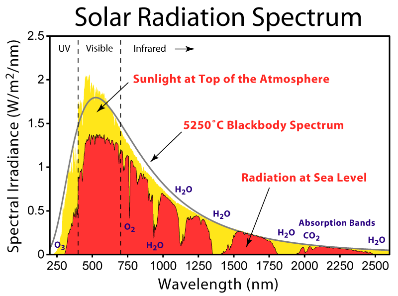
Caption: "This figure shows the solar spectrum for direct light at both the top of the Earth's atmosphere and at sea level. The Sun produces light with a distribution similar to what would be expected from a 5525 K (5250 degrees C) blackbody, which is approximately the Sun's surface temperature. As light passes through the atmosphere, some is absorbed by gases with specific absorption bands. Additional light is redistributed by Rayleigh scattering, which is responsible for the atmosphere's blue color."
Credit/Permission: © Robert A. Rohde (AKA User:Dragons flight), 2007 / Creative Commons CC BY-SA 3.0.
Image linked to Wikipedia.
- Stellar Classification:
The empirical stellar classification is based primarily on stellar spectra.
The most recognizable classification is the OBAFGKM spectral classification (formally the Harvard spectral classification).
Often the OBAFGKM spectral classification is just called the spectral type classification since one refers to the classes as spectral types.
The spectral types run OBAFGKM which is mnemonicked by "O be a fine girl/guy kiss me.".
Caption: A schematic Hertzsprung-Russell (HR) diagram with color index (AKA color) B-V, spectral type along the horizontal axes and absolute magnitude in V. along the vertical axis.
Absolute magnitude in V is a proxy for luminosity (total power integrated over all wavelength).
The bands on the diagram of the luminosity classes are:
-
0 := hypergiants See Wikipedia: List of most massive stars,
where the current record massive star is about 300
M_Suns.
Ia := supergiants
Ib := bright giants
III := giants
IV := subgiants
V := main-sequence stars which are also called dwarf stars, but that now seems a disfavored term.
VI := subdwarf stars
VII := white dwarfs
Credit/Permission: © User:Rursus, 2007 / Creative Commons CC BY-SA 3.0.
Image linked to Wikipedia.
Physically, the OBAFGKM sequence is one of declining photosphere temperature: O stars are hottest, M stars are coldest.
The spectral types are each subdivided into the subtypes 01234569: e.g., a G0 is the hottest G star and a G9 is the coldest G star.
The Hertzsprung-Russell (HR) diagram above correlates spectral types with photosphere temperature and B-V color.
Tables defining the spectral types are at Wikipedia: Spectral types? and Peripatus: Spectral types which seesm better than the Wikipedia one.
- Formation of Absorption Line Spectra:
- Spectroscopes:
Spectroscopes (AKA spectrometers) are devices that disperse light and allow a spectrum to be observed.
The figure below illustrates how a spectroscope works.

Caption: A schematic diagram illustrating how spectroscope or spectrometer works.
The diffraction grating disperses the light.
Credit/Permission: © User:Kkmurray, 2007 / Creative Commons CC BY-SA 3.0.
Image linked to Wikipedia.
In our lab, we use two spectroscopes: Project Star Spectrometer, and WINSCO spectrometer.
It takes some demonstration and playing around with them to see how they work.
The diffraction grating disperses the light according to the diffraction grating formula:
        nλ = d*sin(θ)  ,

             where n is the order number,
             λ is the wavelength,
             d is the spacing between the diffraction grating slits,
             and
             θ is the angle between the normal to the diffraction grating and the interference maximum
                which is the observable.
At the interference maximum, interference is strongly constructive and in between strongly destructive.
The zeroth order diffraction is at θ=0 and there all wavelengths have a maximum.
The intensity of the orders decreases rapidly with order number n.
In this lab, we only look at the 1st order spectral lines.
The diffraction grating formula is usefully rearranged to get
θ(degrees) = arcsin(nλ/d) ≅ (nλ/d)*(180/π) ,where the last formula is a small-angle approximation---which is about 20 % accurate even up to 60 degrees.
From this rearranged diffraction grating formula, it is clear that θ increases with n and λ, and decreases with d.
To get large dispersion, one wants λ/d sufficiently large.
- Gas-Discharge Lamp:
Our sources are an incandescent light bulb (which is soon to be an antique) and a sodium (Na) gas-discharge lamp.
- Clea Stellar Spectra Software:
In this lab, we use Clea Stellar Spectra software The Classification of Stellar Spectra.
Just follow the manual directions and it will all work.
Nota Bene: The right version of The Classification of Stellar Spectra is with the icon VIREO on the desktop, NOT folder 12.


Below are some generic comments for Lab 12: Stellar Spectra that may often apply.
Caption: Film poster for the TheMummy (1932) starring Boris Karloff (1887--1969).
Credit/Permission: Employee or employees of Universal Pictures attributed to Karoly Grosz (fl. 1930s), 1932 (uploaded to Wikipedia by User:Crisco 1492, 2012) / Public domain.
Image linked to Wikipedia.
Any that are semester-section-specific will have to added as needed.
- Some terms have many definitions.
The definitions required for the reports are those that are relevant to astronomy and NOT other topics.
The links given with the lab keywords in Required Lab Preparation are usually better sources than just googling for a term definition. Often googling will lead to the plain wrong definition or a definition by a person who doesn't really understand the term themself and is just paraphrasing someone else's definition.
-
Such a person is a
lexicographer:
-
Lexicographer:
A writer
of dictionaries;
a person who busies himself in tracing the original, and detailing the signification of
words;
a harmless drudge. (Slightly edited.)
- Answer questions that require sentences with sentences.
Usually it is obvious what those questions are.
Sometimes maybe not. Err on the side yes sentences are needed.
Sentences begin with a capital letter letter and end with a period. Usually there is a subject and a verb. Not always.
Since you are working in groups, you should have different group members read over the sentence answers to see if they are correct and comprehensible. Read them out loud.
- There are questions that imply that an explanation must be given
and NOT just a bare yes or no.
So give the explanation NOT just yes or no.
Usually it is obvious what those questions are. Sometimes maybe not. Err on the side yes an explanation is needed.
- Just copying someone else's answer could give you the wrong answer.
Check to see if it is right.
At least check to see if you have copied correctly. Careless copying leads to lousy answers.