| Crystal Structure Prediction and its Application in Earth and Materials Sciences |
| Crystal Structure Prediction and its Application in Earth and Materials Sciences |
For a given potential function  , minimization of energy can be performed in many ways. In this section two general methods are described. Since x is a vector in the multi-dimensional space, the methods would only locate the minimum ‘closest’ to the initial sampling point.
At any given point in configuration space, the internal energy may be expanded as a Taylor series:
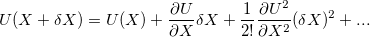 |
(47) |
This expansion is usually truncated at either first or second order, since close to the minimum energy configuration we know that system will behave harmonically. If the expansion is truncated at first order then the minimization just needs the energy term and its first derivatives, which can be done by steepest desecents and conjugate gradient methods 60.
This method assumes the optimum direction to move from the starting  is just the steepest-descent direction g,
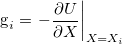 |
(48) |
It is assumed that g can be otained from the negative of a gradient operator  acting on so that
 |
(49) |
Therefore, the next step is,
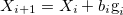 |
(50) |
The step length  can be determined by
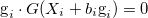 |
(51) |
This method is easy to program, but it often converges slowly. Although each iteration of the steepest-decent algorithm moves the trial vector towards the minimum of the function, there is not guarantee that the minimum will be reached in a finite number of iterations. If the initial steepest-descent vector does not lie at the right angles, a large number of steps will be needed.
![\includegraphics[scale=0.8]{chapter2/pdf/Fig3.png}](images/img-0158.png)
If the only information one has about the function is its value and gradient at a set of points, the optimal method would allow one to combine this information so that each minimization step is independent of the previous ones. To accomplish this, one can derive the condition that makes each minimization step independent of another, the direction of each step should be conjugate to each other.
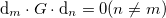 |
(52) |
The precise search direction can be obtained from the following algorithm:
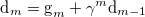 |
(53) |
where
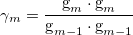 |
(54) |
and  = 0.
= 0.
The initial direction is taken to be the negative of the gradient at the starting point. A subsequent conjungate direction is then constructed from a linear combination of the new gradient and the previous direction that minimized  . Since the minimization along the conjugate directions are independent, the dimensionality of the vector space explored is reduced by 1 at each iteration.
Above I just introduced two most fundamental optimization algorithms. If we expand the energy to second order, the second derivative matrix (Hessian matrix,  ) is needed. In this case, several methods, like Newton-Raphson, Davidon-Flecher-Powell and Broyden-Fletcher-Goldfarb-Shanno can work efficiently 61.
| Crystal Structure Prediction and its Application in Earth and Materials Sciences |